Fitting Lévy Distributions
Because the Lévy distribution has large tails, the variance (expectation of \(x^2\)) is infinite. That means there is no simple way to estimate its parameters from a sum of squares. Instead, we can use Bayesian fitting.
First, we’ll need some data. For this example, I pulled the monthly closing values of the S&P500 index from Yahoo Finanace:
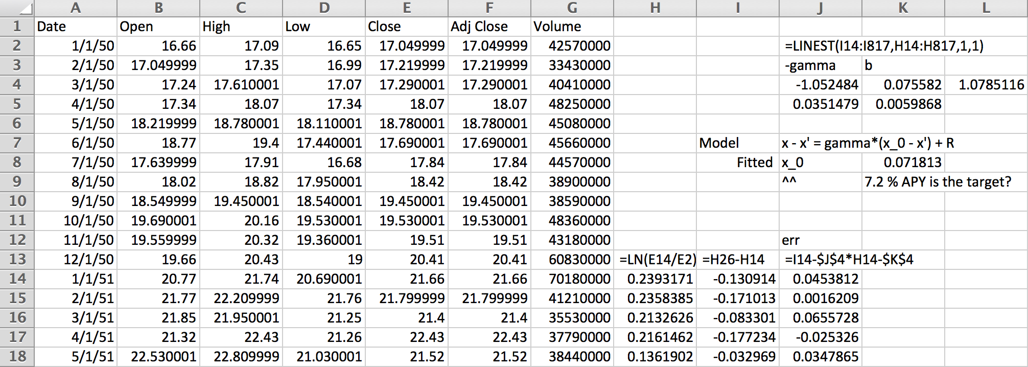
Working on a yearly basis, we get 12 data points per year. The logarithms in column H are essentially continuous compounding market return rates. Predicting next year’s return from last year’s requires fitting column I given column H. The linear regression at the top does this with,
$$ \log(x_{t+1}/x_t) = \gamma (\bar x - \log x_t) + R_t $$
for some zero-mean random increments, \(R_t\). The coefficients show a relaxation rate of nearly 1, which means we may as well have used an AR(0) model that ignores the previous year.
The errors, \(R_t\) are shown in the following histogram:
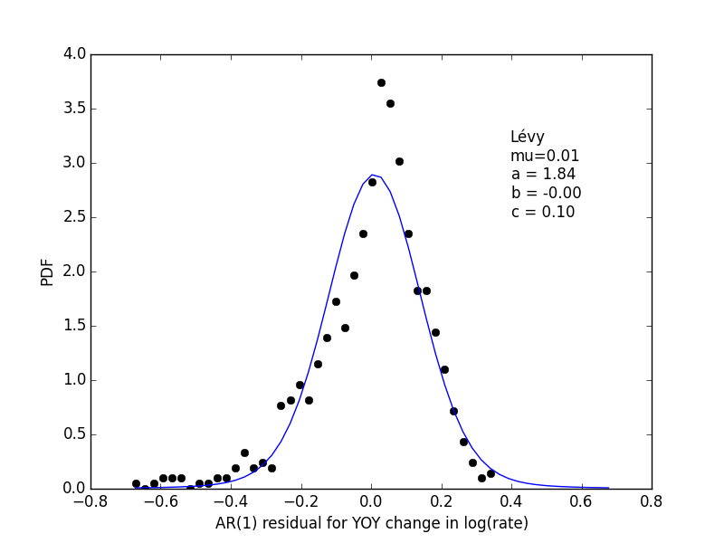
The fitted parameters don’t have a lot of skew like the histogram data points, but are really the maximum likelihood Bayesian estimate. For details, see below.
Plotting the Lévy distribution
The Lévy distribution plot should come from scipy, but
my version shows NotImplementedError. So, I coded
up a manual integration of the Fourier transform like so,
from numpy import *

def levy(y, a, b=0, c=1.0, Npts=2000):
    dp = 0.01
    p = linspace(-10.0, 10.0, Npts)
    dp = p[1]-p[0]

    u = abs(p)**a
    u = u.astype(complex128)
    if b != 0:
        s = ones(len(p))
        s[:100] = -1.0
        if a == 1.0:
            u *= 1.0 + 2j*b/pi * s * log(abs(p/c))
        else:
            u *= 1.0 - 1j*b * s * tan(0.5*pi*a)

    return dot(exp(-1j/c * y[...,newaxis]*p), exp(-u)).real * dp/(2*pi*c)
Fitting the histogram
After saving the residuals to sp500.dat, I created
a histogram using numpy and did some test plots
to get initial paramater estimates.
The function lprob computes the log-posterior,
and using fmin produced a stable answer.
It uses the histogram directly rather than the points
to lower the number of points where levy is computed
– even though it’s probably not too bad either way here.
from scipy.optimize import fmin
import pylab as plt

h = histogram(read_matrix("sp500.dat"), 40)

x = h.lowerlimit + arange(.5, 40.5)*h.binsize
n = h.count
def lprob(mu, a, b, c):
    lp = log(levy(x-mu, a, b, c))
    return dot(n, lp) - log(c)

mu = 0.0
a = 1.5
b = -1.0
c = 0.08
f = lambda v: -lprob(v[0], v[1], v[2], v[3])
v = fmin(f, array([mu, a, b, c]))
print v
print -f(v)
mu, a, b, c = v[0], v[1], v[2], v[3]

x = h.lowerlimit + arange(.5, 53)*h.binsize
pdf = n/float(sum(n))/h.binsize
plt.plot(x[:40], pdf, 'ko')
plt.plot(x, levy(x-mu, a, b, c))
plt.text(0.4, 2.5, u"Lévy\nmu=%.2f\na = %.2f\nb = %.2f\nc = %.2f"%(mu,a,b,c))
plt.gca().set_xlabel("AR(1) residual for YOY change in log(rate)")
plt.gca().set_ylabel("PDF")
plt.savefig("sp500_levy.png")
plt.show()
All in all, I’m a little disappointed that the max-likelihood answer doesn’t have the skew I would have expected.