The Bellman Equation
So lately, I’ve been trying to determine if there’s an exact, mathematically optimal way to make saving and spending decisions. The simple answer was given in the post on Consumption Function Analysis. It says that you should spread out your spending evenly and increase it regularly at the market rate. Unfortunately, it does not take into account any uncertainty inherent in chasing a market rate that is higher than inflation.
Before I start, I should note that the earlier, simple formula can be improved significantly and applied in practice by doing the following:
- Add up all income you will receive over the rest of your lifetime, not counting increases for inflation, and counting only after-tax income.
- Break that total into two numbers, a smaller, ‘safe bet’ number, and a larger, ‘optimistic’ number.
- Add up all your current yearly expenses in today’s dollars and multiply by your maximum lifespan – no correction for inflation.
- Break that total into two numbers, a smaller, ‘required’ expenses number,
and a larger, ‘comfortable’, number.
- Also, scale up your medical expenses and scale down your mortgage expenses to get a good estimate of a lifetime average.
- Note that if all three (savings, income, and expenses) increase with the same rate of inflation, you can make the complete calculation in today’s dollars.
- Do a reality check. Does your minimum income cover your minimum expenses for your life expectancy?
- If not, it’s time to balance your budget or think about delaying retirement.
- If it’s close and you’re nearing retirement, you’re probably uncertain about social security and medical costs (as you should be). Think about annuities that move with inflation and health insurance options to limit that risk.
- Assuming you fall somewhere in the middle, plan on investing enough to cover your required expenses on low risk assets. The rest is excess income that you can invest at high risk and divide up into annual spending as well. Obviously, you should keep track of these numbers when life events happen and adjust your plans accordingly.
With that, let’s dive into the mathematical analysis. First, the Bellman equation is all about answering the question, ‘How much will \(W_{t+1}\) dollars be worth to me next year, given that the world is in state \(S_{t+1}\)?’ The quantitative answer is some function, \(V_{t+1}(W_{t+1}, S_{t+1})\). What the Bellman equation says is that the value function at the current time is equal to the average value function in the future:
$$ V_t(W_t, S_t) = \max_{C_t} \int \left( V_{t+1}(W_{t+1}, S_{t+1}) + U(C_t) \right) dP(W_{t+1}, S_{t+1} | W_t, S_t, C_t) $$
The integral is over the probability of future wealth, and state of the economy, \( W_{t+1}, S_{t+1} \) given that we make the decision \( C_t \). Since the decision is up to us, we are going to pick the one with maximum expected value.
That being said, there are two extreme cases to be aware of. First, say we are just scraping by, so that there is nothing we really get to decide and \( C_t \) is as much as we can afford. In that case, the Bellman equation degenerates into a way to calculate the expected course of the economy in general. In other words, \(dP(W_{t+1}, S_{t+1} | W_t, S_t, C_t)\) has to contain our model for the economic growth, \( S_{t+1} | S_t \).
The other extreme is where the economic model is perfectly known. The example we started with was that everything grows predictably at the rate of inflation. In that case, we can make decisions without worrying about randomness at all.
In-between, we can take a stochastic process model for the economy and make spending decisions based on it. As individuals, our decisions are mostly decoupled from the economy as a whole, so we don’t have to worry about our spending decisions affecting gross domestic product – we’ll leave that to Gates, Soros, and The Fed.
What I would like to say is that there is a simple stochastic process model for the economy as a system. Unfortunately, there are so many unknowns and pitfalls in trying to predict the economy that even the experts advise us to take expert advice with two grains of salt. Nevertheless, let’s investigate some solutions of the Bellman equation. I wasn’t happy with the Levy distribution fit earlier, so I used the simplest choice,
$$ dP(z = \log(S_{t+1}/S_t))/dz = \frac{ab}{a+b} \begin{cases} e^{-a(m-z)}/a & m > z, \\ e^{-b(z-m)}/b & z \ge m \end{cases} $$
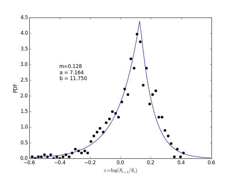
This says the market randomly wins or loses every year with maximum probability at 12.8% return. Its long negative tail makes the average return somewhere around 8%, while the expectation of the appreciated value, \( e^z \), is about 9%. That’s a fairly good gamble, despite the significant risk.
You might ask why the last year’s returns don’t enter the model. It’s hard to believe, but historically, the past year’s returns don’t help predict the next year’s returns much at all – so it’s simpler to ignore them.
Finally, some code:
from numpy import *
from numpy.polynomial.laguerre import laggauss
import pylab as plt

######### create quadrature rules globally ###########
Nquad = 20

# 20-point Gauss-Laguerre quadrature for weight exp(-x) on [0,infty)
# note: 0 is not a quadrature point
x_log, w_log = laggauss(Nquad)

# m, a, b parameters for 2-sided exp distribution
m, a, b = [  0.1279548,   7.16394812, 11.7499037 ]

# create its quadrature array
x_2exp = hstack([ m-x_log[::-1]/a, m+x_log/b ])
w_2exp = hstack([   w_log[::-1]*b,   w_log*a ]) / (a+b)

M = 3 # dimensionality

R1 = 1.03     # risk-free rate
R2 = exp(x_2exp) # market rate (array of possibilities)
quad = lambda z: dot(z, w_2exp)

Year = 1.0
util = lambda c: -1./c
# spending x[2] this year and all market gains next year
V = lambda x: Year*quad(util(R1*x[0,:,:,newaxis] + R2*x[1,:,:,newaxis])) \
                + util(x[2])

W = 100.0
c0, c1 = 45.0, 57.0
r0, r1 = 0.01, 30.0
c = linspace(c0, c1, 100)
rf = linspace(r0, r1, 100)
x  = zeros((3, 100, 100), float)
x[2] = c[:,newaxis]    # spending
x[0] = rf[newaxis,:]   # risk-free investment
x[1] = W - x[0] - x[2] # market investment
plt.imshow(V(x).T, extent=(c0, c1, r0, r1), origin='lowerleft', aspect='auto')
plt.gca().set_xlabel("Spending")
plt.gca().set_ylabel("Bonds")
plt.colorbar()
plt.show()
plt.savefig('value.png')
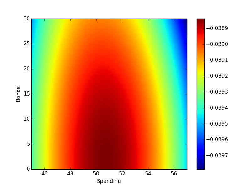
The plot above shows the resulting value function for spending, saving, and investing when you have only 2 years to live with $100,000 in your pocket and the option to buy a 1 year CD for 3% (saving) or invest in the market. Units are thousands of dollars.
Apparently, the maximum expected value is found when spending about $51,000 and throwing the rest into the stock market. Personally, I might not make that choice because of the real risk of taking a 10% loss on the market – leaving only $44,000 in the last year. So we probably need to tweak the value function a bit to distinguish required vs. excess spending.
Of course, repeating this procedure for all starting situations, \(W_t, S_t\), backward to the present will allow making decisions based on the incomplete information we have now. The final conclusion is the common cliche that to do this properly, you really have to know your risk tolerance (that is, what is your utility function?).