Asset Allocation by Convex Optimization

Finally, let’s use the utility function to make a real decision. How much should I invest in the market vs. in a risk-free CD of a given rate?

To make matters concrete, assume this person is living alone and has a terminal illness with precisely 2 years left to live and zero unknown medical expenses (for simplicity). Let’s also say they would greatly prefer to spend above $12,500 per year but only have $23,000 in assets, so there’s likely not enough to pay those bills. This means the market vs. safe assets is a really important choice. Most advisors would say to stick with the safe bet. Let’s see what happens.

Using stock market returns modeled earlier, and utility function from the last post, we compute the negative expected utility and its derivatives using quadrature,

M = 3 # optimization in 3D
R1 = 1.02 # risk-free rate
R2 = exp(x_2exp) # market rates
quad = lambda z: dot(w_2exp, z) # expectation over market rates

C0 = 12.5 # approx 一人 FPL
Year = 1.0
V = lambda x: -quad( Year*util(C0*Year, R1*x[0] + R2*x[1], 0) \
                    + util(C0,x[2],0) )
def dV(x):
    der = Year*util(C0*Year, R1*x[0] + R2*x[1], 1)
    return -array([
        quad( R1*der ),
        quad( R2*der ),
        util(C0, x[2], 1)
     ])
def Hess(x):
    iwp = Year*util(C0*Year, R1*x[0] + R2*x[1], 2)
    ab  = R1*quad(R2*iwp)
    return -array([
           [R1*R1*quad(iwp),    ab, 0.0],
           [ab,    quad(R2*R2*iwp), 0.0],
           [0.0,       0.0, util(C0,x[2],2)]
    ])

Now, we can apply the magic of convex optimization to find an allocation, \( x_0, x_1, x_2 \) = (CDs, stocks, spending), which minimizes negative utility. So we are maximizing

$$ \mathbb E[ U | x_0, x_1 ] + U(x_2) $$ under the constraints \( x_j > 0 \), \( \sum x_j = W \).

Here is the primal-dual optimization Lagrangian, residual, search direction, and backtracking code all in one:

# returns both the primal function and dual (Lagrangian)
def L(v, W):
    x, lm, nu = v[:M], v[M:2*M], v[2*M]
    pri = V(x)
    return pri, pri - vdot(lm, x) + nu*(sum(x)-W)

def resid(v, W, it):
    x, lm, nu = v[:M], v[M:2*M], v[2*M]
    r = zeros(2*M+1)
    r[   :  M] = dV(x)  - lm + nu
    r[  M:2*M] = x*lm   - it
    r[2*M]     = sum(x) - W
    return r

# H = [H, -I, 1]
#     [lm, x, 0]
#     [1,  0, 0]
#
# H*dx - dlm + dnu = -rx
# lm*dx + x*dlm = -rlm
#   => dlm = -(rlm+lm*dx) / x
# (H+lm/x)*dx + dnu = -rx - rlm/x
# 
# [Hp, 1] . [dx ] = -[rx + rlm/x]
# [1,  0]   [dnu]   -[rnu       ]
#
# Hp = H + lm/x

# Determine the pd search direction by solving
# an M+1 dimensional reduced Hessian system.
# validated with:
#    H = num_diff(lambda u: resid(u, it), v)
#    dx2 = la.solve(H.transpose(), -resid(v, it))
#    dx2 == pd_search(v, it)
def pd_search(v, W, it):
    x, lm, nu = v[:M], v[M:2*M], v[2*M]

    # Compact residual:
    r = zeros(M+1)
    r[:M] = dV(x) + nu - it/x
    r[M]  = sum(x) - W

    # Compact Hessian:
    H = zeros((M+1, M+1))
    H[:M,:M] = Hess(x)
    for i in range(M):
        H[i,i] += lm[i]/x[i]
    H[:M,M] = 1.0
    H[M,:M] = 1.0

    dxnu = la.solve(H, -r)
    dv = zeros(2*M+1)
    dv[   :  M] = dxnu[:M]
    dv[  M:2*M] = (it - dxnu[:M]*lm)/x - lm # dlm
    dv[2*M]     = dxnu[M]
    return dv

def gap(x, lm):
    return vdot(x, lm)

def fmin(x, W, eps=1e-8):
    assert M == len(x)
    mu = 10.0

    lm = ones(M)*0.1
    nu = 100.0
    v = zeros(2*M+1)
    v[:M], v[M:2*M], v[2*M] = x, lm, nu

    it = gap(v[:M], v[M:2*M])/(mu * M)
    rnorm = lambda u: sqrt(sum(resid(u, W, it)**2))
    err = rnorm(v)
    step = 0
    #print "step, norm, gap, f(x), L(v), v"
    while err > eps and step < 100:
        step += 1
        fx, Lx = L(v, W)
        #print "%4d %.2e %.2e %.2f %.2f %.2f %.2f %.2f"%(step, err, it*mu*M, fx, Lx, v[0], v[1], v[2])

        dv = pd_search(v, W, it)
        t = min(min( (-v[:M]   /dv[:M])[     where(dv[:M] < 0.0)].min(),
                     (-v[M:2*M]/dv[M:2*M])[where(dv[M:2*M] < 0.0)].min()
                   )*0.99,
                1.0)
        #print v + t*dv
        #print t,
        err2 = rnorm(v+t*dv) # simple backtrack
        while err2 > (1-0.05*t)*err:
            #print err
            t *= 0.5
            err2 = rnorm(v+t*dv)
        #print t
        v += t*dv
        err = err2

        it = gap(v[:M], v[M:2*M])/(mu * M)
        err = rnorm(v) # TODO: correct old err with new it

    fx, Lx = L(v, W)
    return v[:M], v[2*M], fx, Lx, err

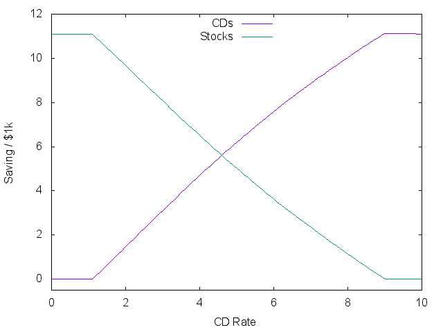
Running this over a set of ‘risk-free’ rates provides the following plots,

for r in arange(101)*0.1:
    R1 = 1.0 + r*0.01
    W = 23.0
    w, nu, fx, _, err = fmin(array([0.9*W, 0.1*W, 0.1*W]), W)
    print("%f %f %f %f %f"%(r, w[0], w[1], w[2], fx))

Saving	Expected Spending

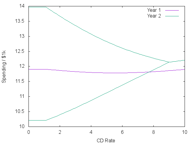The plots show three stages. At the lowest rates, a constant gamble is made on the market market independent of the rate! The two lines on the right show the average plus/minus one standard deviation of what returns might result next year.

As rates go above 1%, there is a real trade-off between risk and reward. Money shifts to safety, while spending in the first year actually goes down to try and capture more rewarding spending next year. Eventually, the risk-free rate is better than historic market returns, and all investments go into bonds. The plots look roughly similar when starting with more cash, but the first stage disappears.

Interestingly, even at high rates without risk, less money is spent during the first year than the second because this will result in more spending overall. In most economic models, future spending is discounted using an ‘immediacy factor’ to scale down this effect.