The utility function expresses personal preferences by mapping from dollars spent into relative happiness. It can help you say ‘meh’ by precisely identifying the locus of events for which you are equally happy (or unhappy) about. A previous post about the Bellman equation used a \(-1/c\) utility function. That was unrealistic because it doesn’t take into account the fact that there is actually a minimum set of costs that everyone faces. For example, the federal poverty level for an individual was $12,140 last year, while that for a family of 4 was $25,100. This article develops a better utility function with a minimum spending preference.

The central idea is to use the 'maximum term approximation' from statistical mechanics: $$ \max(x(t),y(t)) \approx \log( e^{x(t)} + e^{y(t)} ) $$ .

In a molecular context, this equation could describe the dependence of the free energy on temperature, \(t\), during a phase change. Then, \(x\) and \(y\) would both be concave functions giving the free energy of one particular phase. At the boiling point, the operative function switches over from the liquid to the gas curve. This equation also appears in a Bayesian context, where the cross-over represents an abrupt change in opinion between two alternative hypotheses.

In our case, let's use two lines, crossing at \( t = 1\) and shifted so that \(x(0) = 0\): $$ x(t) = \alpha t $$ $$ y(t) = t + \alpha - 1 $$

Now, we can think about replacing the ‘consumption’ argument to the utility function, \(U(C)\), with:

$$ \tilde C(t = C/C_0) = \log(1 + e^{-y(0)}) - \log(e^{-x(t)} + e^{-y(t)}) $$

This inverts the max function to get the min function, and shifts the result so that \( \tilde C(0) = 0 \). The resulting \(\tilde C(t)\) looks like we’d expect (black line):

For the general utility function which grows like the \(1 - \rho\) power of \(C\), we add a scale and shift so that the function crosses zero at \( C_0 \), and has a slope of 1 there.

$$ U(\tilde C) = \frac{C_0}{1-\rho} ({\tilde C(C/C_0)}^{1-\rho} - {\tilde C(1)}^{1-\rho}) $$

Of course, \( \rho = 1\) is a special case.

I’m rather happy with the result, shown for \(\rho = 1, \alpha = 10\):

The two lines are the final utility as a function of dollars spent when your family size is two (blue line) or four (black line).

The code is below:

from numpy import *
import pylab as plt

# constants
rho = 1
C0fac = 10.0
Cmin = log(1.0 + exp(1.0-C0fac))
C0p  = C0fac + Cmin - log(2.0) # zero level
# Assume C0 == 1, since we scale so that dU/dC = 1 at C = C0
# Argument to the utility function is:
# C' = min(C0fac*C, C + C0fac - 1)
# two lines cross at C = 1.0
def util(Cscale, C, n): # for rho != 1
    C = C/Cscale
    C1 = C + C0fac-1 # min
    C2 = C1 - C0fac*C     # diff. (< 0)
    if isinstance(C, ndarray):
        w1 = where(C < 1.0)
        C1[w1] = C0fac*C
        C2[w1] *= -1.0
    elif C < 1.0:
        C1 = C0fac*C
        C2 *= -1.0

    Z  = 1.0/(1.0 + exp((C0fac-1)*(C-1.0)))
    Cp = C1 + Cmin - log(1.0 + exp(C2)) # -log(Z) = x - log(1 + e^{x-y})
    #return Cp # min function

    if n == 0:
        if rho == 1:
            return Cscale*(log(Cp) - log(C0p))
        return (Cp**(1.0-rho) - C0p**(1.0-rho)) * (Cscale/(1.0-rho))
    elif n == 1:
        r = Cp**(-rho)
        return r*(1.0 + (C0fac-1.0)*Z)
    elif n == 2:
        rp = Cp**(-rho)
        rpp = -rho * Cp**(-rho-1.0)
        return (rpp*(1.0 + (C0fac-1.0)*Z)**2 - \
                 rp*Z*(1.0-Z)*(C0fac-1.0)**2 ) / Cscale
    return None

Note how C1 is always the minimum of the two lines, and how C2 stores their difference. This ensures numerical stability, since it isolates the largest contribution (the straight line) and all the log/exp stuff is just a perturbation that goes away far from crossover. I’ve seen codes from respected folks in statistical mechanics that are sloppy, and miss that.

In the next article, I’ll provide the constrained optimization code needed to solve asset allocation problems.

It’s interesting to philosophize a bit at this point. Since the curve seems to say that spending $58,000 on a family of 4 provides a reward of +5 as opposed to cutting back expenses to $19,000 (reward of -5). This makes a great case for charity if we value the spending of others as much as ourselves. Economic data says average charity donations are around $2,000 per year, while median incomes are $54,000. Would donations be higher if we knew the people we could be helping well enough to value their spending?

As much fun as it is predicting the market and risk-free rates based on the economic cycle, the level of US national debt creates a large, worldwide uncertainty that the economic cycle can be understood based on past market data at all. Of course, acting on long-term expectations of the economic cycle should tend to even it out, so the uncertainty I’m mentioning also helps contribute to the cycle in the first place.

Its no secret that the Fed actively manages the yield curve to set ‘risk-free’ interest rates. Although conspiracy theorists disagree, the Fed sets its policy to try and prevent long-term financial crises, so the uncertainty I am talking about here is whether or not the Fed will be successful in its efforts.

From Sept. 2008 to Dec. 2014, the amount of the US national debt increased dramatically as we began ‘quantitative easing,’ which is more or less printing money to cover our government’s spending. That is why we, as a country, have been able to run post losses in the neighborhood $800 Billion per year for the past 10 years.

What is strange is that the rest of the world has continually been encouraging us to overspend. In 1971, President Nixon decided to let that happen by ending the gold standard. The gold standard was an international understanding that the one ounce of gold should be worth about $35 USD. Since people are naturally ingeneous, innovations and technology keep growing at an exponential pace. That means there will usually by many more goods on the market next year than this year, and we will either have to inflate the money supply or else see the price of common goods fall every year.

Psychologically, it’s hard to see sales and wages fall, so we needed inflation. That was impossible under the gold standard, so we ended it. Developing economies, however, tend to make their first steps toward growth by producing goods at low wages for export to developed nations. As their own economies develop, however, their wages go up and it becomes increasingly hard to sell to the US. Enter inflation. As long as our money supply inflates, the government can hand out money in military spending (including overseas aid), retirement and health programs (and interest paid to US banks). Those folks can then spread the money around and eventually all our prices go up. This presents foreign markets with a choice – either raise prices and see slowed economic growth and job loss or else continue working at low wages to sell to the US. They seem to choose to continue selling. Their prices and wages rise too (so they still inflate) but with a lag. Effectively, it is a tax imposed by established economies on every country that wants to use exports for growth. It is the same ‘inflation’ tax we pay at home.

Unfortunately, it creates a mounting problem for us. The accumulated debt acts like a reservoir for possible future inflation. In the beginning of our republic, we had the option to monetize all our debts. Since its start in 1913, the Federal Reserve (a union of banks) appropriated the power to create money as too dangerous for politicians to control, leaving the federal government with only the rights to create new debt instead. However, the idea that new debts will one day be paid in full has become unfashionable even in the business world, where the usual expectation is that all debts will be rolled over, forever. Why give up money when you already have it and things are going well?

Like those businesses, we are continually growing our money supply on one side, while growing our interest payments on the other. If gross domestic production keeps up, then we will grow our capacity to pay, and we can make the system balance out by growing mostly in sync. Yes, we will still have inflation internally, but hopefully inflation plus income taxes can remain tolerable. If, however, we issue too many new debts, then it will become hard to keep up – as anyone considering bankruptcy knows.

Since 2014, the percent of debt owned by foreign countries has been steadily decreasing, presenting a conundrum. The developing world is catching up and is beginning to tolerate slower economic growth in exchange for higher wages. This should be good news.

However, as early as 2014, warning lights started blinking when we awoke to discover that the Federal Reserve system itself owned 64% more US government debt than China. The rapid pace of quantitative easing pushed us higher in debt much faster than we had hoped, making us grey-haired before our time.

So, the big question staring us down is, “How do we remove all this play money from the Fed.’s balance sheet?” I think we need some real financial hocus pocus here, since we can’t afford to keep paying interest on it, while market movements at the end of 2018 showed that we can’t try to pay it off either (since then deflation would happen). I’m not an economist, but I can’t see why other countries would care whether we make interest payments to ourselves or not. So, ideally, the portion of debt held by The Fed itself would disappear. The market is acting as if this were the case.

What the Fed was trying to do (and what markets fear most) is to demand payment of the debt from US taxpayers. If that happens, the US markets will deflate and make it harder to buy imports again. The rest of the world seems to be willing to tolerate some of that. However, the deflation that results will lower stock market prices and cause a Wall St. generated recession. Two things are for sure, we will be squeezed as much as possible on every side and markets will go wherever the Fed wants them to. In that light, it’s interesting to note that Goldman Sachs says there’s a 25% chance of increase and 20% chance of decrease in 2019, some traders have bet big that losses won’t be larger than 22% over 2 years, while Morgan Stanley thinks GDP will decline, forcing a short-term 7% drop.

So lately, I’ve been trying to determine if there’s an exact, mathematically optimal way to make saving and spending decisions. The simple answer was given in the post on Consumption Function Analysis. It says that you should spread out your spending evenly and increase it regularly at the market rate. Unfortunately, it does not take into account any uncertainty inherent in chasing a market rate that is higher than inflation.

Before I start, I should note that the earlier, simple formula can be improved significantly and applied in practice by doing the following:

1. Add up all income you will receive over the rest of your lifetime, not counting increases for inflation, and counting only after-tax income.
2. Break that total into two numbers, a smaller, ‘safe bet’ number, and a larger, ‘optimistic’ number.
3. Add up all your current yearly expenses in today’s dollars and multiply by your maximum lifespan – no correction for inflation.
4. Break that total into two numbers, a smaller, ‘required’ expenses number, and a larger, ‘comfortable’, number.
   • Also, scale up your medical expenses and scale down your mortgage expenses to get a good estimate of a lifetime average.
5. Note that if all three (savings, income, and expenses) increase with the same rate of inflation, you can make the complete calculation in today’s dollars.
6. Do a reality check. Does your minimum income cover your minimum expenses for your life expectancy?
   • If not, it’s time to balance your budget or think about delaying retirement.
   • If it’s close and you’re nearing retirement, you’re probably uncertain about social security and medical costs (as you should be). Think about annuities that move with inflation and health insurance options to limit that risk.
7. Assuming you fall somewhere in the middle, plan on investing enough to cover your required expenses on low risk assets. The rest is excess income that you can invest at high risk and divide up into annual spending as well. Obviously, you should keep track of these numbers when life events happen and adjust your plans accordingly.

With that, let’s dive into the mathematical analysis. First, the Bellman equation is all about answering the question, ‘How much will \(W_{t+1}\) dollars be worth to me next year, given that the world is in state \(S_{t+1}\)?’ The quantitative answer is some function, \(V_{t+1}(W_{t+1}, S_{t+1})\). What the Bellman equation says is that the value function at the current time is equal to the average value function in the future:

$$ V_t(W_t, S_t) = \max_{C_t} \int \left( V_{t+1}(W_{t+1}, S_{t+1}) + U(C_t) \right) dP(W_{t+1}, S_{t+1} | W_t, S_t, C_t) $$

The integral is over the probability of future wealth, and state of the economy, \( W_{t+1}, S_{t+1} \) given that we make the decision \( C_t \). Since the decision is up to us, we are going to pick the one with maximum expected value.

That being said, there are two extreme cases to be aware of. First, say we are just scraping by, so that there is nothing we really get to decide and \( C_t \) is as much as we can afford. In that case, the Bellman equation degenerates into a way to calculate the expected course of the economy in general. In other words, \(dP(W_{t+1}, S_{t+1} | W_t, S_t, C_t)\) has to contain our model for the economic growth, \( S_{t+1} | S_t \).

The other extreme is where the economic model is perfectly known. The example we started with was that everything grows predictably at the rate of inflation. In that case, we can make decisions without worrying about randomness at all.

In-between, we can take a stochastic process model for the economy and make spending decisions based on it. As individuals, our decisions are mostly decoupled from the economy as a whole, so we don’t have to worry about our spending decisions affecting gross domestic product – we’ll leave that to Gates, Soros, and The Fed.

What I would like to say is that there is a simple stochastic process model for the economy as a system. Unfortunately, there are so many unknowns and pitfalls in trying to predict the economy that even the experts advise us to take expert advice with two grains of salt. Nevertheless, let’s investigate some solutions of the Bellman equation. I wasn’t happy with the Levy distribution fit earlier, so I used the simplest choice,

$$ dP(z = \log(S_{t+1}/S_t))/dz = \frac{ab}{a+b} \begin{cases} e^{-a(m-z)}/a & m > z, \\ e^{-b(z-m)}/b & z \ge m \end{cases} $$

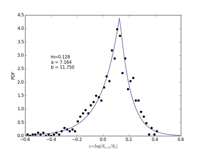
This says the market randomly wins or loses every year with maximum probability at 12.8% return. Its long negative tail makes the average return somewhere around 8%, while the expectation of the appreciated value, \( e^z \), is about 9%. That’s a fairly good gamble, despite the significant risk.

You might ask why the last year’s returns don’t enter the model. It’s hard to believe, but historically, the past year’s returns don’t help predict the next year’s returns much at all – so it’s simpler to ignore them.

Finally, some code:

from numpy import *
from numpy.polynomial.laguerre import laggauss
import pylab as plt

######### create quadrature rules globally ###########
Nquad = 20

# 20-point Gauss-Laguerre quadrature for weight exp(-x) on [0,infty)
# note: 0 is not a quadrature point
x_log, w_log = laggauss(Nquad)

# m, a, b parameters for 2-sided exp distribution
m, a, b = [  0.1279548,   7.16394812, 11.7499037 ]

# create its quadrature array
x_2exp = hstack([ m-x_log[::-1]/a, m+x_log/b ])
w_2exp = hstack([   w_log[::-1]*b,   w_log*a ]) / (a+b)

M = 3 # dimensionality

R1 = 1.03     # risk-free rate
R2 = exp(x_2exp) # market rate (array of possibilities)
quad = lambda z: dot(z, w_2exp)

Year = 1.0
util = lambda c: -1./c
# spending x[2] this year and all market gains next year
V = lambda x: Year*quad(util(R1*x[0,:,:,newaxis] + R2*x[1,:,:,newaxis])) \
                + util(x[2])

W = 100.0
c0, c1 = 45.0, 57.0
r0, r1 = 0.01, 30.0
c = linspace(c0, c1, 100)
rf = linspace(r0, r1, 100)
x  = zeros((3, 100, 100), float)
x[2] = c[:,newaxis]    # spending
x[0] = rf[newaxis,:]   # risk-free investment
x[1] = W - x[0] - x[2] # market investment
plt.imshow(V(x).T, extent=(c0, c1, r0, r1), origin='lowerleft', aspect='auto')
plt.gca().set_xlabel("Spending")
plt.gca().set_ylabel("Bonds")
plt.colorbar()
plt.show()
plt.savefig('value.png')

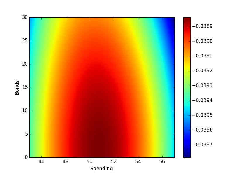
The plot above shows the resulting value function for spending, saving, and investing when you have only 2 years to live with $100,000 in your pocket and the option to buy a 1 year CD for 3% (saving) or invest in the market. Units are thousands of dollars.

Apparently, the maximum expected value is found when spending about $51,000 and throwing the rest into the stock market. Personally, I might not make that choice because of the real risk of taking a 10% loss on the market – leaving only $44,000 in the last year. So we probably need to tweak the value function a bit to distinguish required vs. excess spending.

Of course, repeating this procedure for all starting situations, \(W_t, S_t\), backward to the present will allow making decisions based on the incomplete information we have now. The final conclusion is the common cliche that to do this properly, you really have to know your risk tolerance (that is, what is your utility function?).

Because the Lévy distribution has large tails, the variance (expectation of \(x^2\)) is infinite. That means there is no simple way to estimate its parameters from a sum of squares. Instead, we can use Bayesian fitting.

First, we’ll need some data. For this example, I pulled the monthly closing values of the S&P500 index from Yahoo Finanace:

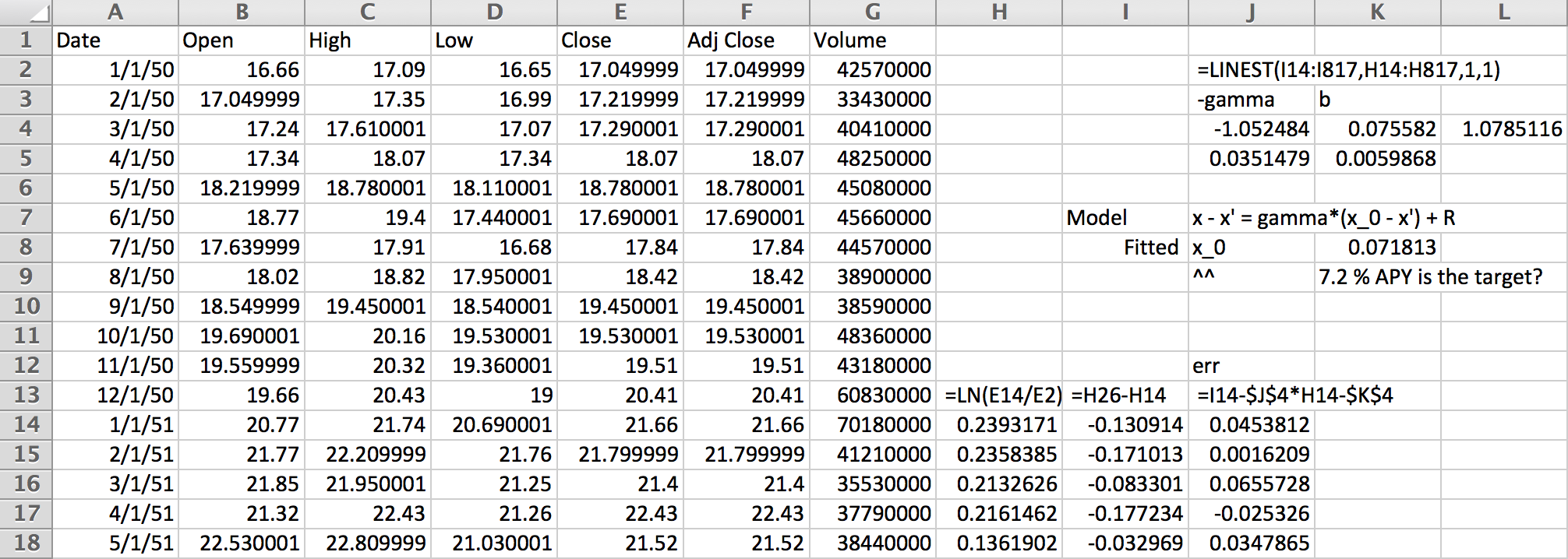
Working on a yearly basis, we get 12 data points per year. The logarithms in column H are essentially continuous compounding market return rates. Predicting next year’s return from last year’s requires fitting column I given column H. The linear regression at the top does this with,

$$ \log(x_{t+1}/x_t) = \gamma (\bar x - \log x_t) + R_t $$

for some zero-mean random increments, \(R_t\). The coefficients show a relaxation rate of nearly 1, which means we may as well have used an AR(0) model that ignores the previous year.

The errors, \(R_t\) are shown in the following histogram:

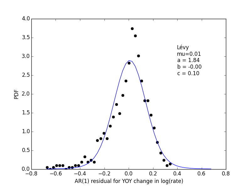
The fitted parameters don’t have a lot of skew like the histogram data points, but are really the maximum likelihood Bayesian estimate. For details, see below.

Plotting the Lévy distribution

The Lévy distribution plot should come from scipy, but my version shows NotImplementedError. So, I coded up a manual integration of the Fourier transform like so,

from numpy import *

def levy(y, a, b=0, c=1.0, Npts=2000):
    dp = 0.01
    p = linspace(-10.0, 10.0, Npts)
    dp = p[1]-p[0]

    u = abs(p)**a
    u = u.astype(complex128)
    if b != 0:
        s = ones(len(p))
        s[:100] = -1.0
        if a == 1.0:
            u *= 1.0 + 2j*b/pi * s * log(abs(p/c))
        else:
            u *= 1.0 - 1j*b * s * tan(0.5*pi*a)

    return dot(exp(-1j/c * y[...,newaxis]*p), exp(-u)).real * dp/(2*pi*c)

Fitting the histogram

After saving the residuals to sp500.dat, I created a histogram using numpy and did some test plots to get initial paramater estimates. The function lprob computes the log-posterior, and using fmin produced a stable answer. It uses the histogram directly rather than the points to lower the number of points where levy is computed – even though it’s probably not too bad either way here.

from scipy.optimize import fmin
import pylab as plt

h = histogram(read_matrix("sp500.dat"), 40)

x = h.lowerlimit + arange(.5, 40.5)*h.binsize
n = h.count
def lprob(mu, a, b, c):
    lp = log(levy(x-mu, a, b, c))
    return dot(n, lp) - log(c)

mu = 0.0
a = 1.5
b = -1.0
c = 0.08
f = lambda v: -lprob(v[0], v[1], v[2], v[3])
v = fmin(f, array([mu, a, b, c]))
print v
print -f(v)
mu, a, b, c = v[0], v[1], v[2], v[3]

x = h.lowerlimit + arange(.5, 53)*h.binsize
pdf = n/float(sum(n))/h.binsize
plt.plot(x[:40], pdf, 'ko')
plt.plot(x, levy(x-mu, a, b, c))
plt.text(0.4, 2.5, u"Lévy\nmu=%.2f\na = %.2f\nb = %.2f\nc = %.2f"%(mu,a,b,c))
plt.gca().set_xlabel("AR(1) residual for YOY change in log(rate)")
plt.gca().set_ylabel("PDF")
plt.savefig("sp500_levy.png")
plt.show()

All in all, I’m a little disappointed that the max-likelihood answer doesn’t have the skew I would have expected.

I have quite a few new programming projects moving lately, and wanted to find a nice code publishing environment to write general notes and documentation on them.

My github profile had been sorely lacking attention for awhile, so I decided to follow their Right Way(TM) instructions for building a nice developer site.

My first thought was “Oh, no! Not another markup language!” since I’ve built a wiki with Wikitext, put together Sphinx documentation with reStructuredText, and used only a bit of markdown. Comparisons out there show that markdown parsed by Ruby’s kramdown are not so bad for code blogs, so what the hey.

Although I followed the basic instructions – which are indispensible for understanding Jekyll’s layout and basic features – the lack of included CSS is painful unless you use a theme.

So, I ploughed all that under and copied a theme from Elena Gong.

So far so good.

Issues

Because my Mac uses fink as a package manager and is a bit old, bundler is not correctly configured and the latest fink-installed ruby and gem binaries are named ruby2.5 and gem2.5, so rvm doesn’t find them with rvm use 2.5 as recommended. Also, an update to libssl I did during development at some point seems to have clobbered some of my ssl certificates, leading to Gem::RemoteFetcher::FetchError: SSL_connect returned=1 errno=0 state=error: certificate verify failed errors.

So, every recommended command using bundler failed. However, when I deleted the Gemfile and manually installed jekyll-paginate, jekyll-seo-tag, etc. (see _config.yml), jekyll build and jekyll serve worked.

Sooner or later I should really fix these packaging issues…