Click here to: start the livestream!

https://youtube.com/live/hmvGq7ThvYs?feature=share

For about four years now, I’ve been learning to play the shakuhachi - on old-school bamboo flute. Here’s a link to my teacher’s website, shawnheadmusic.com, and another to KSK Europe.

Program:

• Yamagoe
• Akita Sugagaki
• Yuyake Koyake
• Sanson no Yugure
• Itsuki no Komoriuta
• Tsuki no Sabaku
• Mushizukiyo
• Kikyou Genso Kyoku
• Kojo no Tsuki

Every day I seem to stumble onto new and interesting scientific computing projects in computational chemistry. They run the gamut from hobby projects and one-off ideas to high-powered science teams with strong followings.

Personally, I suspect the Covid pandemic has driven people to spend more time on computational projects they believe are important and useful. In some sense, it’s nice to work on projects like that. New ideas are worth exploring, but there’s never enough time to try them all.

This article lists some of those projects.

• Real Space Multigrid DFT (RMGDFT)

• DFT-FE

  Two computational chemistry packages for running Kohn-Sham density functional theory. Both have a cmake-based install. RMGDFT has both CPU and GPU versions. DFT-FE uses an energy-level projection method to greatly speed up convergence for metals, and is planning a CUDA-enabled release soon.

• PySCF

• Horton

  PySCF and Horton are python front-ends to libint and libxc. They let you get your hands dirty with Gaussian orbital coefficients for wave-functions. While they can calculate Hartree-Fock orbitals, in my opinion, their real utility is in letting you get at the matrix elements for orbital-orbital interactions. For anyone teaching a modern course in computational chemistry, I’d recommend working these packages into your course material.

• Python Simulation Interface for Molecular Modeling

  This is a set of python scripts for driving polymer simulations with LAMMPS and Cassandra. The research group that developed this is using it regularly to create and simulate hydrocarbon melts with various packing fractions - so I would expect it work very well for this purpose. I had created something like this for a side-project as a postdoc, but never took the time to document, and publish it. Kudos to this group. Disclaimer: I haven’t tested this package.

• DFTB+

  DFTB+ simulates molecules using a tight-binding approximation to the Schrodinger equation. Essentially, it computes energies using quantum mechanics on the valence orbitals only, using simplified orbital shapes. That still puts it in a different leauge than forcefield-based methods, or even AI methods for that matter. I would consider this program great for a simulations project because it’s very well documented and mostly stand-alone, which simplifies the build and install process. Disclaimer: I haven’t tested this package.

• ddcMD

  This program is a highly efficient, barebones, GPU-accelerated MD engine. It is essentially what won the 2020 Gordon Bell special prize for Covid research (by simulating a coarse-grained model of the entire coronavirus). Yes, they narrowly beat out our team… It’s written up in a JCP article. Unfortunately, the code itself is still newly published, so not enough users have nagged them asking for more and better documentation. Go ahead and create an issue!

• Gromacs

  Old programs can learn new tricks, it seems. I added Gromacs to the list here because its recent re-design lets it be used as a python module. Previously, this was accomplished by an external team that wrapped the gromacs library. This is no longer needed! Gromacs has a “gmxapi” python module that is working its way toward providing more APIs that reach into gromacs.

• chemparam

  Finally, a shameless advertisement. The chemparam project creates traditional CHARMM and gromacs forcefield parameter files for small molecules. It uses any ab-initio force data you have on-hand as input to force-matching, which give bond, angle, torsion, and even Lennard-Jones and electrostatic charge parameters. There are some hooks in there to use data from NWChem, but you need some compilation skills and a special patch to get that to work. Of course, it also lets you input force data from your own sources.

Well, that’s been a quick wrap-up of some of the coolest developments I’ve seen lately. Hopefully it can serve as a jumping-off point for your next hobby project.

In some recent work where I’m building a linear algebraic verison of solution density functional theory, I realized that the algebra was quickly getting out of hand. The work neatly shows how to take traditional mathematical methods for working these problems and turn them into numerical methods.

There’s one problem though. The reviewers didn’t see how its result was different from those ancient mathematical ways. To put their fears to rest, I set out to make a few non-traditional numerical implementations of the theory. What I found was that every time I translate the equations to matrices and vectors, I have to consider lots of special cases so that the code quickly becomes littered with ideas that don’t directly translate to equations in the manuscript. This is bad practice, since you don’t want lots of computations without corresponding, documented definitions in your code. There are 2 ways to solve that problem. Either I could make the manuscript significantly larger, or I could write a compiler taking high-level equations and automagically cranking out implementation code.

The second approach is more elegant, and is exemplified by the FEniCS project. There, code like dE = 0.5*eps*inner(nabla_grad(phi), nabla_grad(phi)) creates a symbolic expression standing in for the electrostatic energy density of a potential field, phi. I say ‘standing in’ for, since the new object, dE just created is a mathematical expression tree – not a real number. The expression tree only says how to do the work. If you want to get a final answer, you have to provide eps and phi on a grid (as a vector or matrix). Then the computer can follow the instructions in the tree step by step to get to the answer.

To see how this can work, I built a simple polynomial class that describes how to multiply and add polynomials of the form:

$$ f(x,y) = \sum_{n,m} c_{n,m} x^n y^m $$

This is a standard form, and can be expanded to a really useful symbolic form by making the definitions:

• Monomial: \( x^n y^m \)
• Coefficient: \( c_{n,m} \)
• Polynomial: Sum of monomials times coefficients.

Each of the definitions above gets represented by its own data structure. Without further ado, my implementation is below:

def applyIter(m, k): # cf Haskell's list monad
    for e in m:
        for j in k(e):
            yield j

# dictionary mapping monomials to coefficient ring
# addition must be implemented for each coefficient
# if there are redundant monomials.
class Polynomial(dict):
    def __init__(self, lst): # merge all keys by addition
        d = {}
        for k, v in lst:
            if d.has_key(k):
                d[k] += v
            else:
                d[k] = v
        dict.__init__(self, d)

    def __mul__(a, b):
        return Polynomial(applyIter(a.iteritems(), \
                    lambda (ai,aj): [(ai*bi, aj*bj) for bi,bj in b.iteritems()]))
    def __add__(a, b): # simple concat
        return Polynomial(applyIter([a.iteritems(), b.iteritems()], \
                    lambda u: u))

class Monomial(tuple):
    def __mul__(a, b):
        return Monomial([i+j for i,j in zip(a, b)])
    def __repr__(self):
        return "Monomial%s"%(tuple.__repr__(self))

def test():
    # 3 x - y
    mx = Monomial([1, 0]) # x^1 y^0
    my = Monomial([0, 1]) # x^0 y^1
    a = Polynomial([(mx, 3.0), (my, -1.0)])
    b = a*a
    print(b)

Running the test() function shows the result:

{Monomial(2, 0): 9.0, Monomial(0, 2): 1.0, Monomial(1, 1): -6.0}

which is the polynomial representing \( 9 x^2 + y^2 - 6 x y\).

If you know the scipy library, you might be asking how this differs from Numpy’s polynomial module. First, I used terminology and concepts from Macaulay2, a special-purpose symbolic algebra package for these kinds of calculations. Second, and more obviously, the representation here is sparse – so that you don’t have to have a vector or matrix of coefficients.

The link with the Macaulay2 project is intentional. In the actual application I’m developing, the monomials are members of a closed, finite symmetry group. Also, the coefficients are radial basis functions rather than numbers. Symbolic algebra with those objects isn’t possible with vanilla polynomials, but will be in my complete code.

Solving the Bellman equation for personal finances provides a way to find ‘optimal’ trajectories that guide spending and saving decisions in the same way NASA guides probes to make a target trajectory through the solar system.

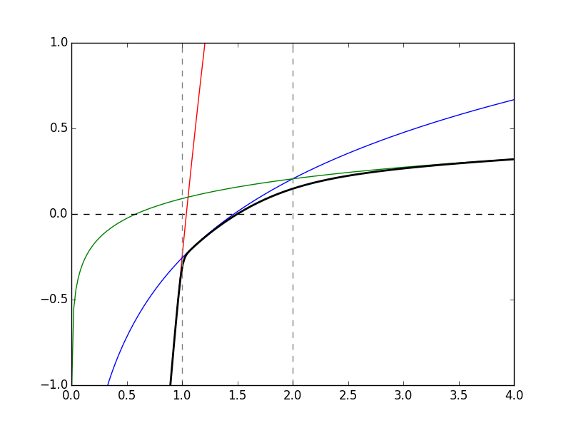
After solving this a few times, I wasn’t happy with the earlier utility function. It always ended up spending at poverty level until it was possible to escape the pull of gravity altogether with wealth flying off to infinity. It might be a good choice for an ascetic, however, for most people, it would be better to tweak the utility function to create three separate segments:

• a steep logarithmic rise below poverty level (FPL)
• a medium logarithmic rise between 1x and 2x FPL
• a slow logarithmic rise above 2x FPL

The graphic is here:

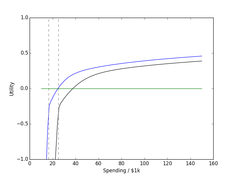
Three Segment Utility (normalized to 1)	Utility for \( C_0 \) = $16,460 and \( C_0 \) = $25,100

and the equation is here:

$$ U(t = C/C_0) = \mathrm{const. } - \log(e^{-A\log t} + e^{-B\log t - y_0} + e^{-C\log t - z_0})/B $$ where \( y_0 = A \log(1) - B \log(1) \) and \( z_0 = B \log(2) + y0 - C \log(2) \) are determined by the fixed crossing points, \( C = 1 \) and \( C = 2\).

I also added a constant to the utility function so that it crosses zero at \( C = 1.5 C_0 \), 1.5 times the minimum spending. I’ve been able to get by just fine spending less than 1.5x the FPL, so it’s probably a good target. Note that this is a spending target, not an income target - since income at the FPL is an unsustainable living condition.

I chose to work backward from a ‘final’ utility function at age 90 based on \( C_0 \) = $5,000 in today’s dollars, representing the low-end cost of a casket funeral. The utility function above targets 1 to 2x this amount, so tries to attain between $5,000 and $10,000 – also reasonable.

I used the median household income of $59,055 to guestimate a starting salary of $55,000 for an average household that starts work at 22 years of age. I didn’t add $55,000 as income though, but rather added 85% of that to account for taxes and other witholdings that inevitably disappear – possibly never to be seen again. The plots below also assume the interest rate on savings stays at 3.4 and inflation is 3.56. It also assumes income grows at 4%, which is just 0.5% after inflation. All numbers are inflation-adjusted to Jan., 2019 dollars. I also planned for the following events:

• annual minimum costs of $25,100 from age 18 until 42
• Early retirement at age 55
• Two children at age 22 and 23 (extra medical expenses of $2,000 each)
• ‘donations’ of $20,000 to each child at age 18

• annual minimum costs of $16,460 from 42 onward (2-person household)

  Yes, I know this isn’t a lot to donate to college tuition, but they should be applying to scholarships and dealing with their own finances, shouldn’t they? Also, there is negative cash flow between ages 18 and 22, since they should be studying instead of working. In my model, students have to deal with being financially unhappy because of that. In reality, they will take out loans and pay them off as part of their spending over the next 5-10 years.

  With all that background, let’s examine the ‘value function,’ \( V_t(W, R) \) that results. Since the function is a sum over all years from \( t \) until 90, I’ve divided through by years remaining to show the yearly average in the plot below, so \( \langle U\rangle = V_t(W, R) / (91-t) \). If everything goes ‘on average,’ the trajectory (arrows) would go horizontally to the right, then to the left. In simulations (below), it dips down, then goes up in the most probable cases. The key point is that if \( \langle U\rangle \) goes up with time, the future is getting brighter.

We see that the value function looks roughly logarithmic at every age, but scales and shifts a lot while bending a bit over time. The horizontal axis shows current wealth in 2019 dollars and the vertical axis plots the ‘lifetime average value’ received by a random group of folks at that particular wealth level and age. The curves further to the right (near early retirement at 55) are hurdles, for which one needs significant savings/investments to make it past unscathed. The arrow says a 55-year old retiring today (who knows for certain they will not live past 90) should have nearly $1M in investments.

Oh, I forgot to say above that we’ve vexed our player by putting in a 0.5% chance of losing all job income in any given working year, along with a fluctuating income that can go up or down by 10% from the expectation each year. This idea (and model) comes from Christopher Carroll’s paper I talked about earlier. Formally, the multiplier has a Gaussian distribution with \(\sigma\) = 0.1.

To break this down, let’s contrast it the famous monologue from with Shakespeare’s ‘As You Like It’. The plot above actually shows a financial view of the seven ages of man. If the age divisions are financial, we can even speculate on starting and ending year for each age.

A		With 4 years of zero income ahead, school-boys in this scenario are not looking forward to college unless they have maybe $60,000 saved up. Luckily, most are more wistful than the Bellman equation. This trouble goes away quickly between 18 and 22.
B	The future looks very rosy all around at 22, the age where work begins in this scenario. Regardless of how savings do over the next many years, or how bad college life was, spending can now be high, and future income can take care of any issues.
C		Reality has set in, and expectations are getting higher. This is apparently do or die time. Setbacks here could delay retirement.
D	With savings at maximum, the justice has a lot to loose. It’s only natural those nearing retirement would be concerned with fairness, personal property, and not changing the rules!
E		Let’s say the stage just after retirement belongs to the lean and slippered pantaloon (on the right here). Spending is dialed-in, and the cash flow will be negative for the forseeable future. Still, donations could make up part of that spending.
F	Interestingly, the value curve for second childishness also returns back to almost resemble that for the infant as well…

We should also examine some trajectories that show how a test subject fares when following this advice under random income and investment performance. After making some test trajectories, I realized there was a really strong preference for a 100% stock investment strategy. Everyone knows this is risky, and it turns out that quite a few trajectories crashed and got stuck spending at FPL for the final 10-15 years - ouch.

So… I intervened and capped stocks at 90% of the portfolio unless the current wealth was enough to support $30,000 in spending for each remaining year. This is the recommendation I get from CNN’s asset allocator for even the most risk tolerant, long-term investor. That’s why you can see hard stops at 90% in several plots below – the Bellman equation encourages risky behavior because it’s 50/50 make it big or lose everything at some stages of life.

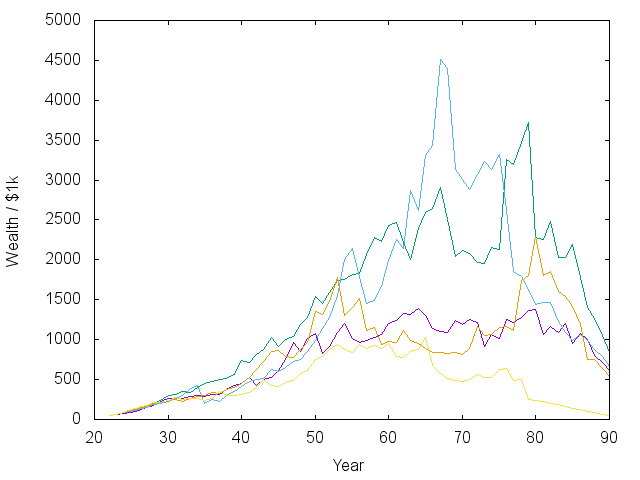
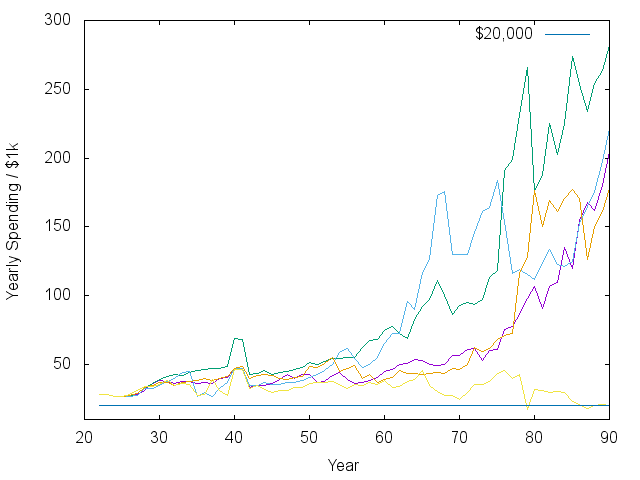
Wealth vs. Time	Spending vs. Time
Expected Average Utility	Investment Strategy

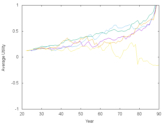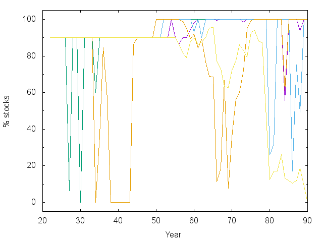With that caveat, I would consider most of the trajectories above successful, showing that it really is possible to retire at 55 on the median income. Note that the spending vs. time plot has already counted for inflation. The exponential rise means an exponential increase in real spending. There is also a noticeable bump and dip in spending as the kids are sent off into the world. I should say that in some other models I did where inflation was not a predictable 3.5%, then it was harder to make steady progress.

Note also that there are periods of large swings in the market and in asset allocation. The model I’m using allows the interest rate on savings to fluctuate – sometimes above 10%. When that happens, like early on in the green and orange lines, the model says to jump into the bond market. Such jumps could contribute to the boom/bust cycle…

Finally, I am not an investment advisor, so don’t take any of this advice without consulting an actual, qualified one. I explicitly disclaim liability for any misfortunes of anyone else based on anything I write down or say!

Finally, let’s use the utility function to make a real decision. How much should I invest in the market vs. in a risk-free CD of a given rate?

To make matters concrete, assume this person is living alone and has a terminal illness with precisely 2 years left to live and zero unknown medical expenses (for simplicity). Let’s also say they would greatly prefer to spend above $12,500 per year but only have $23,000 in assets, so there’s likely not enough to pay those bills. This means the market vs. safe assets is a really important choice. Most advisors would say to stick with the safe bet. Let’s see what happens.

Using stock market returns modeled earlier, and utility function from the last post, we compute the negative expected utility and its derivatives using quadrature,

M = 3 # optimization in 3D
R1 = 1.02 # risk-free rate
R2 = exp(x_2exp) # market rates
quad = lambda z: dot(w_2exp, z) # expectation over market rates

C0 = 12.5 # approx 一人 FPL
Year = 1.0
V = lambda x: -quad( Year*util(C0*Year, R1*x[0] + R2*x[1], 0) \
                    + util(C0,x[2],0) )
def dV(x):
    der = Year*util(C0*Year, R1*x[0] + R2*x[1], 1)
    return -array([
        quad( R1*der ),
        quad( R2*der ),
        util(C0, x[2], 1)
     ])
def Hess(x):
    iwp = Year*util(C0*Year, R1*x[0] + R2*x[1], 2)
    ab  = R1*quad(R2*iwp)
    return -array([
           [R1*R1*quad(iwp),    ab, 0.0],
           [ab,    quad(R2*R2*iwp), 0.0],
           [0.0,       0.0, util(C0,x[2],2)]
    ])

Now, we can apply the magic of convex optimization to find an allocation, \( x_0, x_1, x_2 \) = (CDs, stocks, spending), which minimizes negative utility. So we are maximizing

$$ \mathbb E[ U | x_0, x_1 ] + U(x_2) $$ under the constraints \( x_j > 0 \), \( \sum x_j = W \).

Here is the primal-dual optimization Lagrangian, residual, search direction, and backtracking code all in one:

# returns both the primal function and dual (Lagrangian)
def L(v, W):
    x, lm, nu = v[:M], v[M:2*M], v[2*M]
    pri = V(x)
    return pri, pri - vdot(lm, x) + nu*(sum(x)-W)

def resid(v, W, it):
    x, lm, nu = v[:M], v[M:2*M], v[2*M]
    r = zeros(2*M+1)
    r[   :  M] = dV(x)  - lm + nu
    r[  M:2*M] = x*lm   - it
    r[2*M]     = sum(x) - W
    return r

# H = [H, -I, 1]
#     [lm, x, 0]
#     [1,  0, 0]
#
# H*dx - dlm + dnu = -rx
# lm*dx + x*dlm = -rlm
#   => dlm = -(rlm+lm*dx) / x
# (H+lm/x)*dx + dnu = -rx - rlm/x
# 
# [Hp, 1] . [dx ] = -[rx + rlm/x]
# [1,  0]   [dnu]   -[rnu       ]
#
# Hp = H + lm/x

# Determine the pd search direction by solving
# an M+1 dimensional reduced Hessian system.
# validated with:
#    H = num_diff(lambda u: resid(u, it), v)
#    dx2 = la.solve(H.transpose(), -resid(v, it))
#    dx2 == pd_search(v, it)
def pd_search(v, W, it):
    x, lm, nu = v[:M], v[M:2*M], v[2*M]

    # Compact residual:
    r = zeros(M+1)
    r[:M] = dV(x) + nu - it/x
    r[M]  = sum(x) - W

    # Compact Hessian:
    H = zeros((M+1, M+1))
    H[:M,:M] = Hess(x)
    for i in range(M):
        H[i,i] += lm[i]/x[i]
    H[:M,M] = 1.0
    H[M,:M] = 1.0

    dxnu = la.solve(H, -r)
    dv = zeros(2*M+1)
    dv[   :  M] = dxnu[:M]
    dv[  M:2*M] = (it - dxnu[:M]*lm)/x - lm # dlm
    dv[2*M]     = dxnu[M]
    return dv

def gap(x, lm):
    return vdot(x, lm)

def fmin(x, W, eps=1e-8):
    assert M == len(x)
    mu = 10.0

    lm = ones(M)*0.1
    nu = 100.0
    v = zeros(2*M+1)
    v[:M], v[M:2*M], v[2*M] = x, lm, nu

    it = gap(v[:M], v[M:2*M])/(mu * M)
    rnorm = lambda u: sqrt(sum(resid(u, W, it)**2))
    err = rnorm(v)
    step = 0
    #print "step, norm, gap, f(x), L(v), v"
    while err > eps and step < 100:
        step += 1
        fx, Lx = L(v, W)
        #print "%4d %.2e %.2e %.2f %.2f %.2f %.2f %.2f"%(step, err, it*mu*M, fx, Lx, v[0], v[1], v[2])

        dv = pd_search(v, W, it)
        t = min(min( (-v[:M]   /dv[:M])[     where(dv[:M] < 0.0)].min(),
                     (-v[M:2*M]/dv[M:2*M])[where(dv[M:2*M] < 0.0)].min()
                   )*0.99,
                1.0)
        #print v + t*dv
        #print t,
        err2 = rnorm(v+t*dv) # simple backtrack
        while err2 > (1-0.05*t)*err:
            #print err
            t *= 0.5
            err2 = rnorm(v+t*dv)
        #print t
        v += t*dv
        err = err2

        it = gap(v[:M], v[M:2*M])/(mu * M)
        err = rnorm(v) # TODO: correct old err with new it

    fx, Lx = L(v, W)
    return v[:M], v[2*M], fx, Lx, err

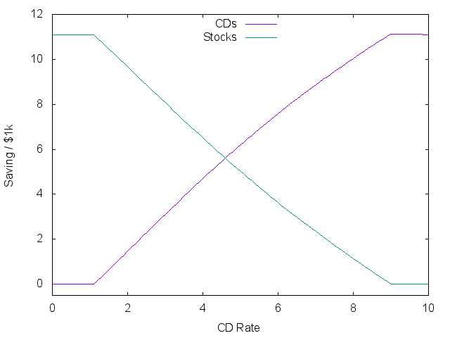
Running this over a set of ‘risk-free’ rates provides the following plots,

for r in arange(101)*0.1:
    R1 = 1.0 + r*0.01
    W = 23.0
    w, nu, fx, _, err = fmin(array([0.9*W, 0.1*W, 0.1*W]), W)
    print("%f %f %f %f %f"%(r, w[0], w[1], w[2], fx))

Saving	Expected Spending

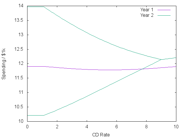The plots show three stages. At the lowest rates, a constant gamble is made on the market market independent of the rate! The two lines on the right show the average plus/minus one standard deviation of what returns might result next year.

As rates go above 1%, there is a real trade-off between risk and reward. Money shifts to safety, while spending in the first year actually goes down to try and capture more rewarding spending next year. Eventually, the risk-free rate is better than historic market returns, and all investments go into bonds. The plots look roughly similar when starting with more cash, but the first stage disappears.

Interestingly, even at high rates without risk, less money is spent during the first year than the second because this will result in more spending overall. In most economic models, future spending is discounted using an ‘immediacy factor’ to scale down this effect.